Build a Footprint Indicator

Volume footprint data shows what standard candlestick charts hide: the exact distribution of buying and selling pressure at each price level within a bar. Professional traders use footprint analysis to identify the Point of Control, spot where institutional orders cluster, and read volume delta at specific prices. Pine Script v6 makes this accessible to every TradingView developer through the request.footprint() function¹.

This tutorial walks through building a complete footprint overlay indicator from scratch. By the end, you will have an indicator that plots POC boundaries, Value Area High and Low levels, and labels showing buy volume, sell volume, and delta on every bar. Each step builds on the last, so you can follow along in the Pine Editor and see results as you go.

What We Are Building

The finished indicator overlays four key levels on each chart bar and attaches a volume information label. Here is what each component does:

• POC Upper and Lower lines mark the price boundaries of the Point of Control row, the row with the highest total volume in the bar
• Value Area High (VAH) line marks the upper boundary of the range where a specified percentage of total volume traded
• Value Area Low (VAL) line marks the lower boundary of that same range
• A label above each bar displays the total buy volume, sell volume, and volume delta

The POC levels are plotted as solid step lines so they stand out on the chart. The VAH and VAL levels use dotted lines to distinguish them from the POC. Together, these levels give you an immediate visual read on where the volume concentrated within each bar and the directional pressure at those levels.

Step 1: Indicator Declaration

Every Pine Script indicator starts with a version annotation and an indicator() call. Since our footprint indicator overlays price data, we set overlay to true. We also set max_labels_count to a reasonable value so the volume labels display across enough bars.

//@version=6
indicator("Volume Footprint Overlay", overlay = true, max_labels_count = 500)

The max_labels_count parameter controls how many label objects can exist on the chart at once. The default is 50, which is too few for a label-per-bar indicator². Setting it to 500 gives you coverage across a wide range of visible bars without hitting memory limits.

Step 2: User Inputs

The indicator needs two user-configurable settings that control how the footprint data is structured. These inputs map directly to the parameters of request.footprint().

// --- Inputs ---
int ticksInput = input.int(100, "Ticks per row", minval = 1,
     tooltip = "Price range of each footprint row in ticks. Smaller values = finer granularity.")
float vaInput  = input.float(70.0, "Value Area %", minval = 1.0, maxval = 100.0, step = 5.0,
     tooltip = "Percentage of total volume that defines the Value Area. Industry standard is 70%.")

Ticks per row determines the height of each price row in the footprint. A tick is the smallest price increment for the symbol, defined by syminfo.mintick². If a stock has a mintick of 0.01 and you set ticks_per_row to 100, each row spans one dollar of price. For futures like ES with a mintick of 0.25, setting ticks_per_row to 4 gives one-point rows.

Value Area % sets what percentage of total volume defines the Value Area. The 70% default is the industry standard used by most market profile and footprint tools. Increasing this value widens the Value Area boundaries. Decreasing it narrows the focus to the most concentrated zone of activity.

Step 3: Request Footprint Data

With the inputs defined, we can make the footprint data request. The request.footprint() function returns a footprint object ID containing all the volume data for the current bar, or na if no footprint data is available².

// --- Footprint Request ---
footprint reqFootprint = request.footprint(ticksInput, vaInput)

This single call retrieves pre-calculated volume data from TradingView's data feeds. Before this function existed, developers had to approximate footprint data by requesting intrabar prices with request.security_lower_tf() and manually sorting volume into price buckets³. The native function is faster, more accurate, and uses only one request call.

There are two important constraints to keep in mind. First, only TradingView Premium and Ultimate plan subscribers can use request.footprint()². Scripts containing this call will not compile on lower-tier plans. Second, each script can contain only one unique request.footprint() call². If you need different ticks_per_row configurations, you must use separate indicators.

Step 4: Extract POC and Value Area

The footprint object by itself is just a container. To extract the data we need, we pass its ID to the built-in footprint.*() functions. These return volume_row objects for key price levels and numeric values for aggregate volume metrics².

// --- Extract Key Rows and Volume Data ---
// Only process if footprint data is available for this bar.
float pocUpperPrice = na
float pocLowerPrice = na
float vahUpperPrice = na
float valLowerPrice = na
float buyVolume     = na
float sellVolume    = na
float deltaVolume   = na

if not na(reqFootprint)
    // Get volume_row objects for key levels.
    volume_row pocRow = footprint.poc(reqFootprint)
    volume_row vahRow = footprint.vah(reqFootprint)
    volume_row valRow = footprint.val(reqFootprint)

    // Extract price boundaries from each row.
    pocUpperPrice := pocRow.up_price()
    pocLowerPrice := pocRow.down_price()
    vahUpperPrice := vahRow.up_price()
    valLowerPrice := valRow.down_price()

    // Get aggregate volume metrics for the entire footprint.
    buyVolume  := footprint.buy_volume(reqFootprint)
    sellVolume := footprint.sell_volume(reqFootprint)
    deltaVolume := footprint.delta(reqFootprint)

We declare all the output variables as na before the conditional block. This ensures the plots display nothing on bars where footprint data is unavailable, which can happen on the earliest bars in the chart's history or on symbols that do not support footprint data.

Inside the if block, three calls to footprint.poc(), footprint.vah(), and footprint.val() retrieve the volume_row objects for the Point of Control, Value Area High, and Value Area Low rows respectively². Each volume_row object holds the data for one specific row within the footprint.

We then call volume_row.up_price() and volume_row.down_price() on each row to get the upper and lower price boundaries². For the POC, we extract both boundaries to plot a visible band. For the VAH, we only need the upper price. For the VAL, we only need the lower price. This gives us the four price levels that define the key zones of the footprint.

Finally, footprint.buy_volume(), footprint.sell_volume(), and footprint.delta() return the aggregate volume values for the entire bar². The delta is the difference between buy and sell volume. A positive delta means more buying pressure. A negative delta means more selling pressure.

Step 5: Plot the Levels

Now we plot the extracted price levels on the chart. The POC boundaries use solid step lines in a bold color to mark the most important level. The Value Area boundaries use dotted lines in a subtler color to frame the volume concentration zone without visual clutter.

// --- Plot POC Boundaries ---
plot(pocUpperPrice, "POC Upper", color.new(color.orange, 0), 2, plot.style_stepline)
plot(pocLowerPrice, "POC Lower", color.new(color.orange, 0), 2, plot.style_stepline)

// --- Plot Value Area Boundaries ---
plot(vahUpperPrice, "VA High", color.new(color.blue, 30), 1, plot.style_stepline_diamond)
plot(valLowerPrice, "VA Low",  color.new(color.blue, 30), 1, plot.style_stepline_diamond)

We use plot.style_stepline for the POC boundaries because step lines create a clear horizontal level at each bar without diagonal connections between bars². This matches how footprint levels actually work: each bar has its own independent POC that does not smoothly transition to the next bar's POC.

For the Value Area lines, plot.style_stepline_diamond adds small diamond markers at each step, making them visually distinct from the POC lines even at a glance. The 30% transparency on the blue color keeps these lines visible but secondary to the POC.

When footprint data is not available for a bar, the variables hold na, and the plot functions automatically display nothing. No additional conditional logic is needed.

Step 6: Add Volume Labels

The final component is a label on each bar that displays the volume breakdown. This gives you a quick numerical read without needing to hover over anything or open a separate panel.

// --- Volume Information Labels ---
if not na(reqFootprint) and barstate.isconfirmed
    color deltaColor = deltaVolume >= 0 ? color.green : color.red
    string footprintInfo = str.format(
         "B: {0,number,#.##}\nS: {1,number,#.##}\nD: {2,number,#.##}",
         buyVolume, sellVolume, deltaVolume
     )
    label.new(bar_index, high, text = footprintInfo,
         yloc = yloc.abovebar, style = label.style_none,
         textcolor = deltaColor, size = size.small)

Each label shows three lines of information. B is the total buy volume. S is the total sell volume. D is the volume delta. The label color reflects the delta direction: green for positive delta (more buying) and red for negative delta (more selling). This color coding lets you scan across bars and immediately see the directional flow.

We use barstate.isconfirmed to create labels only on confirmed bars. Without this check, labels would be created on every tick of the current realtime bar, resulting in duplicate labels stacking on top of each other. On historical bars, barstate.isconfirmed is always true, so all historical bars get labels³.

The label.style_none setting removes the label's background box and pointer arrow, leaving only the text floating above the bar. This keeps the chart clean when you have hundreds of labels visible.

Complete Code

Here is the full indicator combining all the steps above into a single script you can paste directly into the Pine Editor.

//@version=6
indicator("Volume Footprint Overlay", overlay = true, max_labels_count = 500)

// --- Inputs ---
int ticksInput = input.int(100, "Ticks per row", minval = 1,
     tooltip = "Price range of each footprint row in ticks. Smaller values = finer granularity.")
float vaInput  = input.float(70.0, "Value Area %", minval = 1.0, maxval = 100.0, step = 5.0,
     tooltip = "Percentage of total volume that defines the Value Area. Industry standard is 70%.")

// --- Footprint Request ---
footprint reqFootprint = request.footprint(ticksInput, vaInput)

// --- Extract Key Rows and Volume Data ---
float pocUpperPrice = na
float pocLowerPrice = na
float vahUpperPrice = na
float valLowerPrice = na
float buyVolume     = na
float sellVolume    = na
float deltaVolume   = na

if not na(reqFootprint)
    volume_row pocRow = footprint.poc(reqFootprint)
    volume_row vahRow = footprint.vah(reqFootprint)
    volume_row valRow = footprint.val(reqFootprint)

    pocUpperPrice := pocRow.up_price()
    pocLowerPrice := pocRow.down_price()
    vahUpperPrice := vahRow.up_price()
    valLowerPrice := valRow.down_price()

    buyVolume  := footprint.buy_volume(reqFootprint)
    sellVolume := footprint.sell_volume(reqFootprint)
    deltaVolume := footprint.delta(reqFootprint)

// --- Plot POC Boundaries ---
plot(pocUpperPrice, "POC Upper", color.new(color.orange, 0), 2, plot.style_stepline)
plot(pocLowerPrice, "POC Lower", color.new(color.orange, 0), 2, plot.style_stepline)

// --- Plot Value Area Boundaries ---
plot(vahUpperPrice, "VA High", color.new(color.blue, 30), 1, plot.style_stepline_diamond)
plot(valLowerPrice, "VA Low",  color.new(color.blue, 30), 1, plot.style_stepline_diamond)

// --- Volume Information Labels ---
if not na(reqFootprint) and barstate.isconfirmed
    color deltaColor = deltaVolume >= 0 ? color.green : color.red
    string footprintInfo = str.format(
         "B: {0,number,#.##}\nS: {1,number,#.##}\nD: {2,number,#.##}",
         buyVolume, sellVolume, deltaVolume
     )
    label.new(bar_index, high, text = footprintInfo,
         yloc = yloc.abovebar, style = label.style_none,
         textcolor = deltaColor, size = size.small)

Add this script to any chart with a TradingView Premium or Ultimate plan and you will immediately see the POC band, Value Area boundaries, and volume labels overlaid on your price bars.

Customization Ideas

The base indicator provides a solid foundation. Here are several ways to extend it for more advanced analysis.

Highlight Volume Imbalances

Use footprint.rows() to iterate through every row in the footprint and check volume_row.has_buy_imbalance() or volume_row.has_sell_imbalance()². Draw boxes or change the background color when imbalances cluster, signaling strong directional conviction.

// Example: Flag bars with buy imbalances at the POC
if not na(reqFootprint)
    volume_row pocRow = footprint.poc(reqFootprint)
    if pocRow.has_buy_imbalance()
        label.new(bar_index, low, "BUY IMB",
             yloc = yloc.belowbar, style = label.style_label_up,
             color = color.green, textcolor = color.white, size = size.tiny)

Add a Delta Histogram

Plot the volume delta as a histogram in a separate pane to visualize the directional flow over time. Combine it with the overlay to see both the price levels and the aggregate flow in one view.

POC Migration Tracking

Compare the current bar's POC price to the previous bar's POC price to track whether the heaviest volume is migrating up or down. This gives you a directional bias signal that many order flow traders rely on.

// Example: Detect POC migration direction
float prevPocMid = (pocUpperPrice[1] + pocLowerPrice[1]) / 2
float currPocMid = (pocUpperPrice + pocLowerPrice) / 2
bool pocRising  = currPocMid > prevPocMid
bool pocFalling = currPocMid < prevPocMid

Filter by Time Session

Wrap the footprint analysis in a session filter using time() so the indicator only shows footprint levels during regular trading hours. This is especially useful for futures and forex instruments where overnight volume can distort the profile.

Automate Footprint Strategies

Footprint data is powerful for identifying high-probability trade setups. When the POC shifts direction, the delta confirms the move, and price holds above the Value Area Low, you have a confluence signal that many institutional traders use to enter positions.

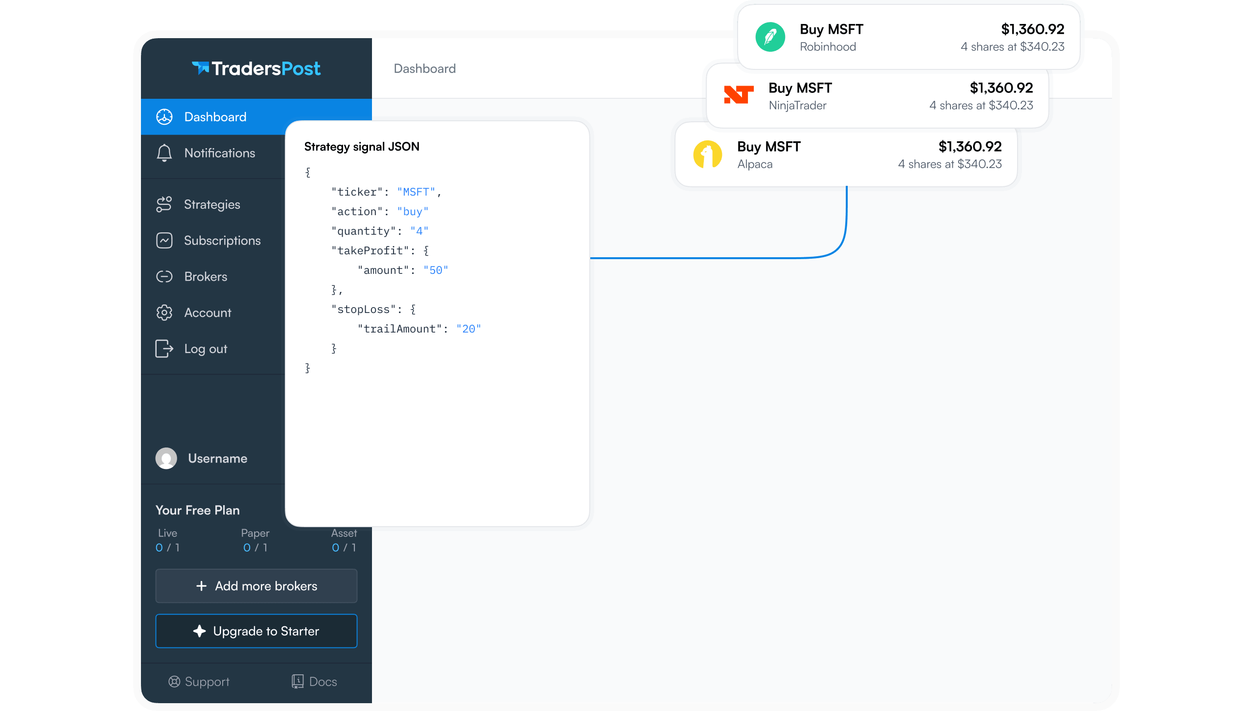
With TradersPost, you can convert footprint-based Pine Script strategies into automated trades. Set up a TradingView alert on your footprint strategy, connect it to TradersPost via webhook, and TradersPost will route the order to your broker automatically⁴. This lets you capture footprint signals around the clock without watching the screen.

Whether you trade futures, stocks, or crypto, connecting a footprint strategy to TradersPost means your analysis translates directly into execution. You build the logic in Pine Script, test it on historical data, and then flip the switch to live trading with a single webhook connection.

References

¹ Pine Script Release Notes
² Pine Script v6 Language Reference
³ Pine Script User Manual
⁴ TradersPost — Automated Trading Platform