Correlated Pairs Trading: Identification Guide
Learn to identify tradeable correlated pairs using cointegration, the Engle-Granger test, z-score entries, and a cost-aware screening workflow.

Marketing

Correlated pairs trading is one of the most mis-specified strategies in retail quant finance. Traders screen for high correlation, find two stocks that move together, and build a spread trade, only to discover the spread drifts indefinitely rather than reverting. The problem is that correlation is the wrong filter. The tradeable property in a pairs strategy is cointegration, not correlation, and distinguishing the two correctly determines whether the strategy has a statistical edge at all.
This guide walks through the Engle-Granger cointegration procedure, the multiple-testing trap that inflates false positives when screening large universes, how to anchor lookback windows to the half-life of mean reversion, and how to set z-score entry and exit rules. It closes with cost modeling and a sequential screening workflow that separates pairs worth paper trading from statistical noise.
Correlation vs. Cointegration
Why correlation misleads traders
Correlation measures whether two price series move in the same direction over a given window, but a high correlation coefficient says nothing about whether the spread between them is bounded. Two trending series can show near-perfect correlation even when their spread drifts permanently apart. A long-short entry based on a correlation-identified pair is therefore built on a non-stationary spread, which has no reliable mean to revert to.
Correlation is also a static snapshot that collapses when the sampling window changes. A pair that looks tightly linked at a weekly frequency can look uncorrelated at a daily frequency. This instability means a high correlation reading at one point in time gives little information about whether the spread will behave predictably going forward.
What cointegration adds
Cointegration says that a linear combination of two integrated series is itself stationary. In practical terms, the spread has a tendency to return to a stable mean rather than wander indefinitely. That mean-reversion property is precisely what makes the spread tradeable: entries are taken when the spread deviates from its mean, and exits occur when it reverts.
Crucially, two series can be weakly correlated in returns yet strongly cointegrated in levels. Correlation in returns and cointegration in levels are measuring different things. That is why the cointegration test, not the correlation coefficient, is the correct filter for identifying pairs candidates.
The Engle-Granger Procedure
Step one: confirm both series are I(1)
The Engle-Granger method requires both price series to be integrated of order one: non-stationary in levels but stationary in first differences. An augmented Dickey-Fuller test applied to each series in levels, and then to first differences, confirms this I(1) status before any cointegration test is run. Running the cointegration test on series that are not I(1) produces meaningless output, so this pre-check is not optional.
Step two: run the cointegration test
The statsmodels.tsa.stattools.coint function implements the augmented Engle-Granger two-step test: regress one series on the other with a constant, then test the residuals for a unit root using an augmented Dickey-Fuller test.1 The null hypothesis of coint is no cointegration; a p-value below the chosen threshold allows rejection of that null, supporting the inference that a cointegrating relationship exists.1
The function returns a t-statistic, a MacKinnon approximate p-value, and critical values at the 1%, 5%, and 10% levels based on the number of observations, per MacKinnon 1994.1
Step three: save the hedge ratio
The regression coefficient from the first stage is the hedge ratio: it defines how many units of the second instrument offset one unit of the first. The spread used in all subsequent analysis is computed as Y minus the hedge ratio times X. Recalculating this ratio periodically is necessary because the relationship can drift over time; a stale ratio causes the spread to be mismeasured and z-scores to be biased.
The Multiple-Testing Trap
How false positives accumulate
A universe of 500 stocks produces 124,750 unique pairs. At a 5% significance threshold, running the cointegration test across all of them will flag thousands of pairs as cointegrated even when no true relationships exist in the data. The raw p-value from any single test is not interpretable without an adjustment for the number of tests performed.
Applying a Bonferroni correction or a Benjamini-Hochberg false-discovery-rate adjustment tightens the effective threshold but does not eliminate the problem when the universe is large. Corrections shift the statistical threshold; they do not raise the underlying prior probability that a genuine relationship exists.
Restricting the universe on economic grounds
The only filter that genuinely raises the prior probability of a cointegrating relationship is restricting the candidate universe using economic reasoning before any test is run. Natural candidate groups include sector peers with shared cost structures, an ETF and its component stocks, dual-listed shares of the same company, and commodity futures on closely related underlyings.
Starting from a small, economically motivated set and then applying a statistical test produces far fewer spurious positives than screening a broad universe and trying to correct for multiplicity afterward. Economic logic and statistical testing should work in sequence, not as substitutes.
Choosing the Right Lookback
Half-life of mean reversion
The half-life of mean reversion, estimated by fitting an AR(1) model to the spread, tells you approximately how many periods the spread takes to decay halfway back to its mean. A spread whose half-life is longer than your intended holding period is not practically tradeable even if the Engle-Granger test statistic is strong, because reversion will not occur within the window you can hold the position.
Half-life also sets a natural lower bound on the lookback window used to estimate the mean and standard deviation of the spread. Using a window shorter than a few half-lives produces a noisy estimate that will generate erratic z-score signals regardless of how strong the underlying cointegration is.
Lookback stability and regime sensitivity
A lookback that spans multiple market regimes may include a period when the pair was cointegrated and a period when it was not, diluting both the test statistic and the spread statistics. Walk-forward testing with rolling windows of different lengths is the standard way to assess how sensitive the hedge ratio and spread mean are to lookback choice. When estimates change materially across adjacent windows, the cointegrating relationship is likely unstable and the pair should be downweighted or excluded.
Z-Score Entry and Exit Rules
Computing the z-score
The z-score of the spread is the spread minus its rolling mean, divided by its rolling standard deviation, calculated over a window calibrated to the half-life. A z-score above a positive threshold signals the spread is stretched to the upside: short the first instrument and buy the second in proportion to the hedge ratio. A z-score below a negative threshold signals the reverse.
Entry thresholds and exit rules
Common entry thresholds sit at plus or minus 1.5 to 2.0 standard deviations. Tighter thresholds generate more signals but with lower average expected reversion per trade, so the per-trade gross return shrinks precisely when cost pressure is highest.
Exit rules should close the position when the z-score reverts to zero, not when it reaches the entry threshold on the opposite side. Waiting for a full mean cross captures the complete reversion move. A stop-loss triggered when the z-score exceeds plus or minus 3.0 standard deviations limits tail exposure when the spread fails to revert and instead enters a new regime.
Automating entries and exits via webhook
Once a Pine Script or external process computes the spread z-score and fires an alert at the entry and exit thresholds, each leg of the pairs trade can be sent as a separate webhook payload using the ticker and action fields. TradersPost also accepts a root-level JSON array of signals when the Allow batch signals setting is enabled in strategy settings, so both legs can be submitted in a single webhook request rather than sequentially.
The Cost Check Most Screens Skip
Two-sided transaction costs
Every pairs trade involves four executions: entering and exiting both legs. Commissions, exchange fees, and bid-ask spread on each leg must be summed across all four fills to arrive at total round-trip cost. The bid-ask spread component is often larger than the commission component for liquid equities, and it scales with the number of shares or contracts traded per leg.
Gross expected reversion per trade must comfortably exceed total round-trip cost before a pair is worth running. A strong cointegration statistic that leaves minimal margin after costs is not a viable strategy, regardless of how low the Engle-Granger p-value is.
Slippage and market-impact estimates
Market orders on both legs simultaneously can move the price of less liquid instruments, adding implicit cost not captured by historical quoted spreads. Using limit orders reduces market impact but introduces execution risk: if one leg fills and the other does not, the resulting single-leg position is an unhedged directional trade. Realistic cost modeling requires historical bid-ask data at the times of hypothetical entries, not just closing prices, to avoid overstating net returns in backtests.
Correlation Breakdown: The Main Risk
Why pairs relationships fail
Cointegrating relationships are not permanent. Structural changes such as a merger, a regulatory shift, or a fundamental divergence in business model can cause a previously stable spread to drift without reverting. A widening z-score that does not revert within the expected half-life is the early warning sign that the relationship may have broken down rather than presenting a better entry opportunity.
The statsmodels documentation notes that if two series are almost perfectly collinear, the test is numerically unstable, though in that degenerate case they are cointegrated under the maintained I(1) assumption.1 Outside that edge case, the more common failure mode is a genuine structural break that the test cannot detect in real time.
Monitoring and position limits
Re-running the cointegration test on a rolling basis and flagging pairs whose p-value has risen above the acceptance threshold provides a systematic way to exit relationships that have deteriorated. Position-level stop-losses set at a z-score of 3.0 or beyond act as a circuit breaker when the statistical monitoring lags the structural break.
Running multiple pairs from the same sector simultaneously concentrates risk in sector-level shocks that can widen all spreads at the same time. Cross-pair correlation of spread returns should be assessed before allocating capital, because the diversification benefit across sector peers is lower than it appears from looking at each pair in isolation.
A Workable Order of Operations
Screening workflow summary
The sequence matters as much as any individual step. Start with an economically motivated candidate list, confirm I(1) status on each series, run the Engle-Granger test with a conservative threshold adjusted for the number of tests, estimate the half-life, reject pairs whose half-life exceeds the target holding period, then model round-trip costs against expected gross reversion. Only pairs that clear every filter in sequence warrant further investigation.
- Economically motivated candidate list, before any test
- I(1) confirmation on both series via augmented Dickey-Fuller
- Engle-Granger test with a multiple-comparison-adjusted threshold
- Half-life estimate; reject if half-life exceeds holding period
- Round-trip cost model against expected gross reversion per trade
- Document hedge ratio, lookback, entry and exit z-score thresholds, and stop level before going live
Statistical significance alone is insufficient justification for live trading. A pair can pass the cointegration test and still be economically untradeable once costs and practical holding-period constraints are applied.
Paper trading before live deployment
Running the strategy in a paper environment allows verification that webhook signals for both legs arrive and fill as expected before real capital is at risk. Paper trading also surfaces execution sequencing issues, such as one leg filling significantly later than the other, that backtests on historical close prices cannot reveal. TradersPost supports paper trading across stocks, futures, options, and crypto, making it practical to run the full pairs workflow in simulation before connecting a live broker account. Start there, confirm both legs route correctly on every signal, and only then move to live execution.
Bottom Line
- Correlation measures co-movement; cointegration measures whether the spread is stationary. Only the second property supports a pairs trade.
- The Engle-Granger procedure requires I(1) confirmation first, then tests residuals for a unit root; the returned p-value and critical values are based on MacKinnon 1994 approximations.1
- Screening 500 stocks generates 124,750 pairs; restrict the universe on economic grounds before running any test, not afterward.
- Anchor the lookback window to several half-lives of mean reversion; reject pairs whose half-life exceeds your realistic holding period.
- Model four-execution round-trip costs against expected gross reversion before treating any pair as tradeable.
Frequently Asked Questions
What is the difference between correlation and cointegration in pairs trading?
Correlation measures co-movement in returns over a window and can be high even when the price spread drifts permanently apart. Cointegration means a linear combination of the two price series is stationary, so the spread has a bounded, mean-reverting character that is actually tradeable. Pairs strategies require cointegration because reversion to a stable mean is the mechanism that generates any expected profit.
How do I choose a lookback window for the spread calculation?
Estimate the half-life of mean reversion by fitting an AR(1) model to the spread. The lookback window for the spread mean and standard deviation should span several half-lives. A spread whose half-life exceeds your intended holding period is not practically tradeable regardless of how strong the test statistic appears. Test multiple lookback lengths in a walk-forward framework and prefer the length whose hedge ratio and spread statistics are most stable across adjacent windows.
How many pairs should I test to avoid false positives?
Testing a large undifferentiated universe inflates the false-positive rate severely at any standard significance level. Restricting the candidate list on economic grounds before running any statistical test is the most effective way to raise the prior probability of a genuine relationship. If testing more than a handful of pairs, apply a multiple-comparison correction such as Bonferroni or Benjamini-Hochberg to adjust the effective significance threshold.
What z-score thresholds should I use for entry and exit?
Entry thresholds in the range of plus or minus 1.5 to 2.0 standard deviations are common; tighter thresholds increase signal frequency but reduce average expected reversion per trade. Exit should occur when the z-score reverts to zero rather than waiting for it to reach the entry threshold on the opposite side, to capture the full mean-reversion move. A stop-loss at plus or minus 3.0 standard deviations limits exposure when the spread fails to revert and may be entering a regime break.
How do I know if a cointegrated pair has stopped working?
Re-run the Engle-Granger test on a rolling basis; a p-value that has risen above your acceptance threshold signals that the relationship has likely deteriorated. A z-score that widens beyond 3.0 standard deviations without reverting within several half-lives is a practical early warning that the spread may not be mean-reverting anymore. Structural events such as mergers, spin-offs, regulatory changes, or major business model shifts are the most common causes of permanent cointegration breakdown and warrant immediate review of any affected pair.
References
1 statsmodels.tsa.stattools.coint - statsmodels documentation